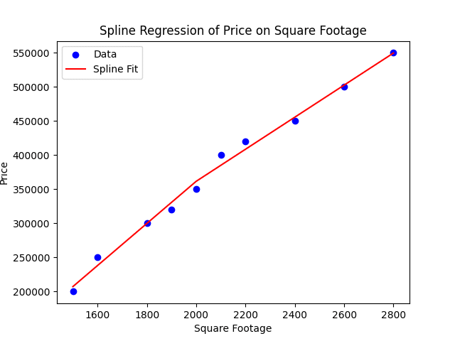
9. You have data on housing prices and square footage and notice that the relationship between square footage and price is nonlinear. Fit a spline regression model to allow the relationship between square footage and price to change at 2,000 square feet. Explain how spline regression can capture different behaviours of the relationship before and after 2,000 square feet.
PROGRAM:
import pandas as pd
import numpy as np
import statsmodels.api as sm
import matplotlib.pyplot as plt

# dataset
data = {
    'Price': [200000, 250000, 300000, 320000, 350000, 400000, 420000, 450000, 500000, 550000],
    'SqFt': [1500, 1600, 1800, 1900, 2000, 2100, 2200, 2400, 2600, 2800]
}
df = pd.DataFrame(data)

# Define the spline term for SqFt with knot at 2000
df['sqft_knot'] = np.maximum(0, df['SqFt'] - 2000)

# Define independent variables (including intercept)
X = sm.add_constant(df[['SqFt', 'sqft_knot']])
y = df['Price']

# Fit linear regression with spline
model = sm.OLS(y, X).fit()

# Print summary
print(model.summary())

# Plot the fitted spline regression
plt.scatter(df['SqFt'], df['Price'], color='blue', label='Data')
plt.plot(df['SqFt'], model.predict(X), color='red', label='Spline Fit')
plt.xlabel('Square Footage')
plt.ylabel('Price')
plt.title('Spline Regression of Price on Square Footage')
plt.legend()
plt.show()OUTPUT:
                            OLS Regression Results
==============================================================================
Dep. Variable:                  Price   R-squared:                       0.992
Model:                            OLS   Adj. R-squared:                  0.990
Method:                 Least Squares   F-statistic:                     458.5
Date:                Wed, 03 Sep 2025   Prob (F-statistic):           3.78e-08
Time:                        08:53:50   Log-Likelihood:                -105.38
No. Observations:                  10   AIC:                             216.8
Df Residuals:                       7   BIC:                             217.7
Df Model:                           2
Covariance Type:            nonrobust
==============================================================================
                 coef    std err          t      P>|t|      [0.025      0.975]
------------------------------------------------------------------------------
const      -2.557e+05   4.11e+04     -6.217      0.000   -3.53e+05   -1.58e+05
SqFt         308.7019     22.587     13.667      0.000     255.293     362.111
sqft_knot    -73.5822     32.468     -2.266      0.058    -150.356       3.191
==============================================================================
Omnibus:                        1.654   Durbin-Watson:                   1.972
Prob(Omnibus):                  0.437   Jarque-Bera (JB):                0.915
Skew:                           0.381   Prob(JB):                        0.633
Kurtosis:                       1.729   Cond. No.                     2.55e+04
==============================================================================

Notes:
[1] Standard Errors assume that the covariance matrix of the errors is correctly specified.
[2] The condition number is large, 2.55e+04. This might indicate that there are
strong multicollinearity or other numerical problems.
